
· By Sajeevan (Saj) Veeriah
Embedded systems · 4 min read
A noisy sensor needs a decision rule
How hysteresis, debounce and explicit states turn a fluctuating measurement into a useful event without hiding the timing cost.
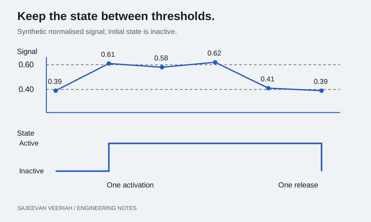
A sensor value sitting near a threshold can cross it repeatedly even when the physical situation has barely changed. If every crossing becomes an event, one movement can turn into several counts.
My embedded assessment device uses Hall-effect sensing to observe movement. The normalised values below illustrate how hysteresis and debounce handle a noisy signal.
Separate the measurement from the event
Keep the raw measurement available during development. A displayed count is the result of several decisions: how the input was sampled, whether it was valid, which state was active, and whether a transition was accepted. Logging only the final count removes the evidence needed to explain a miscount.
Start by defining the event in physical terms. Does it mean entering a detection region, leaving it, or completing a sequence across two sensors? Those definitions lead to different state machines. A single threshold crossing does not automatically tell you direction or distance.
Use hysteresis when the boundary chatters
Hysteresis uses different switching thresholds depending on the current state. Analog Devices describes how separating rising and falling thresholds can prevent repeated switching around a noisy boundary. The same state-dependent idea can be expressed in firmware.
For an illustrative normalised signal, enter the active state at 0.60 or above. Stay active until the signal reaches 0.40 or below. Between those values, retain the previous state. Define the equality cases explicitly so tests at exactly 0.40 and 0.60 have predictable outcomes.
With an initial inactive state, the sequence 0.39, 0.61, 0.58, 0.62, 0.41, 0.39 produces one activation and one release. A single 0.60 threshold would produce two activations and two releases in this sequence. These values demonstrate the rule only; choose real thresholds from measured noise, tolerances and the required operating range.
Sources: [1]
Debounce answers a different question
Debounce asks whether a candidate condition has lasted long enough, or remained present across enough samples, to accept it. Hysteresis separates signal levels; debounce adds a time requirement. Combining them can help, but excessive qualification time can suppress legitimate short events.
Suppose samples arrive exactly every 10 ms and the rule requires five consecutive qualifying samples. The interval from the first qualifying sample to the fifth is 40 ms. For a clean transition occurring at an arbitrary point between samples, acceptance is approximately 40-50 ms later, before scheduling or processing delays.
At 0.2 m/s, that idealised delay corresponds to 8-10 mm of travel. This does not mean the measured position is necessarily wrong by that amount: timestamping and the measurement model matter. It does mean that a delay chosen to make a graph look quiet has a physical consequence.
Write down the states, including invalid input
A compact transition table exposes ambiguity before it becomes firmware. This example uses hysteresis without the optional debounce stage.
| State and input | Decision |
|---|---|
| Inactive; signal ≥ 0.60 | Enter active; emit one activation event. |
| Active; signal ≤ 0.40 | Enter inactive; emit one release event. |
| Valid signal between thresholds | Keep the current state; emit no event. |
| Invalid or stale sample | Mark the measurement invalid; apply a separately defined recovery rule. |
Do not quietly interpret a disconnected sensor as a legitimate zero. Keep validity separate from active or inactive status. On recovery, decide whether a new baseline is required before counting again.
Test where the rule is most likely to fail
Replay recorded raw signals through the decision logic. Include slow crossings, noise near both thresholds, short valid pulses, reversals, startup inside the active region and missing samples. Compare accepted events with independently labelled physical events.
Report false events, missed events and detection delay separately. A configuration that removes false counts by rejecting every event is easy to make and useless in practice. Keep the raw data and the rule version together so a change can be checked against the same evidence.
Sources: [2]
Sources and further reading
Sources checked on 11 September 2026. Signal values and timing calculations are worked examples.